The world of supply chain management is full of experts.

I struggle with the fact that in the Supply Chains to Admire work that we find that global multi-nationals struggle to scale performance. We are not able to achieve economies of scale. I think that one of the reasons is a lack of focus on supply chain fundamentals.

The Dance With Shiny Objects

Many “experts”, I find, dance in the aura of new shiny objects- pontificating on the promise of the autonomous supply chain and touting the power of agentics. I say, let them have it.

“Faster horses?” Here is a quote that I like.

 Users may not always articulate the solution — but they are living with the problem.
And to understand that problem, you need to leave your own assumptions at the door. You need to stop projecting your context onto theirs.
Innovation doesn’t come from asking users what to build.
It comes from deeply understanding what it feels like to be them.

“Faster Horses” — Why Henry Ford Didn’t Say It, and Why We Should Stop Thinking Like He Did | by Karolien François | Medium

If you are struggling with supply chain planning, dancing in the light of shiny objects, and scratching your head, please read on. My goal is to help you.

Drive Value: Rethink Fundamentals

Please do not AI Stupid. What do I mean? AI Stupid is putting agents and agentics on top of existing architectures believing that making them faster and hands free add value. To me, this is fools play.

I love AI. I am excited about new technologies. To this end, I want to shine a light on how new technologies can help address the black holes and inconsistencies in today’s supply chain, which largely stem from the limitations of the first generation of supply chain planning and execution technologies. In this blog, I give you three places to start.

Step One: Align on First-Principle Thinking

In prior blog posts, I asked teams to rethink their processes using first principles and improve their AI readiness.

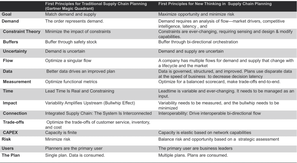
In essence, what is it that you to do anyway, spoken in plain language? To get started, read the first column and then think about the difference in the second column, and ask yourself if this delta is important in your organization. Once clarity is achieved, start a discussion with technologists. Get past the shiny-object bunk and focus on driving value.

Table 1. Supply Chain First Principles

Step 2. Redefine Your Relationship With Data

The second step is to take an inventory of the data you have and ideate possible use cases or opportunities to redefine data structures to reduce latency and improve relevance. Traditional processes have inherent process and data latency that we should no longer accept. I have written many blogs on the need for a planning master data layer and a unified data model in my market-driven research.

Step 3: Embrace and Understand Lead Time

In the supply chain, lead time is a gossamer thread. Lead time should connect and link planning, inventory management, procurement, manufacturing, and customer delivery; getting it right is key to driving supply chain reliability, but in most supply chains it is a broken gossamer.

Gossamer is a light, fine thread web. A broken gossamer is hard to see.

When supply chains become less predictable and difficult to control, supply chain entropy—the accumulation of uncertainty and inefficiency increases. Disorder reigns. Functions within a company are not aligned, and the systems are not interconnected with a consistent and accurate definition of lead time. Supply chain effectiveness requires order and alignment of parameters to actuals.

Whild companies try to put pat answers on the cunundrum like risk management or improving resilience, a lot of progress can be made by focusing on reducing disorder.

Entropy is a measure of uncertainty, disorder, or the number of possible ways a system can be arranged.

Supply chain entropy is related to, but distinct from, the Bullwhip Effect. Let’s not confuse the two. The bullwhip effect describes how small changes in customer demand become amplified and distorted as they move through the supply chain. Entropy is broader, encompassing all sources of increasing disorder. A major source of disorder is the lack of discipline around lead time management. The larger and more complex the organization, the greater the opportunity.

The Opportunity

As a composite metric, aggregate lead time is the total time to complete all cycles: order, replenishment, manufacturing, procurement, and logistics cycles. This varies by item, category, region, asset class, and time period. It should never be a set-it-and-forget-it value. While many leaders speak of dynamic lead times — where lead time values are updated based on actual supply chain data — this is seldom the reality. In this world of increasing variability, it is important to understand the average and variance to drive a predicted lead time. (See Table 2)

Role in Planning Cycles

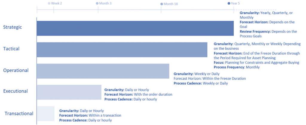
Aggregate lead time defines planning horizons. As shown in Figure 1, planning processes vary and are defined by aggregate lead time. Getting clean on these definitions is a first step toward governance and discipline.

• Tactical Planning. In the tactical horizon—the focus of demand and supply planning and Sales and Operations (S&OP) planning—the emphasis is on planning beyond aggregate lead time.
• Operational Planning. In the operational time horizon, the planning focus is synchronizing and harmonizing data across source, make, and deliver to improve delivery reliability. The operational time horizon includes transportation load tendering, production scheduling, materials requirements planning, distribution requirements planning, and inventory allocation. Lead time also plays a critical role in JIT and VMI processes. Without it, materials never arrive on time.
• Executional Planning. The order cycle time defines the executional planning time horizon and drives the cadence for routing, warehouse management, and inventory deployment.

Figure 1. Lead Time Defines Planning Horizons

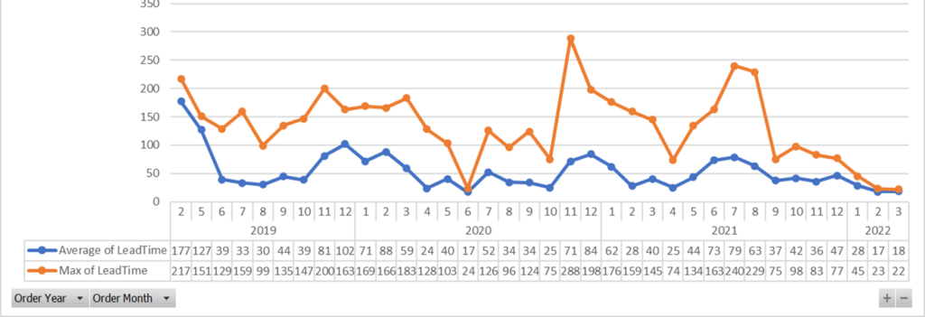
In traditional deployments, lead time was defined by a series of averages. With increased supply variability and the advent of new forms of math and solvers, probabilistic engines use both the average and the pattern of lead time to calculate the probability of lead time included in the aggregate lead time calculation. In Figure 2, we present an example of raw-material inbound lead time for an automotive distributor.

Figure 2. Managing a Supply Chain in a World of Increased Variability

---

Role in Safety Stock

Lead time actuals should be used in the calculation of safety stock. Unfortunately, when we interviewed thirty supply chain professionals, we found that no leader was updating lead time in safety stock calculations based on actuals or using demand variability in their calculations. As a result, many feel comfortable in their safety stock calculations, but they shouldn’t.

To help the reader, here we share one formula used to calculate safety stock (there are many):

Safety Stock = Z × √[(LT × σd²) + (D² × σLT²)]

Where:

• D = average demand per day
• σd = standard deviation of demand
• LT = average lead time
• σLT = standard deviation of lead time

This accounts for variability in both demand and supplier performance.

The So What and Who Cares

So, as you play with shiny objects and talk about the promise of AI, remember, that your current architectures were compromised by the limitations of technologies fifty years ago. As you redefine the promise of planning with new technologies, start with first principles, redefine your relationship with data (to use all forms of data), and put some discipline around the use of lead times. Your supply chain will thank-you.

And if you want to calculate the impact of your current supply chain entropy, in the appendix, I share some formulas. To monetize the affect of entropy on your supply chain, push the insights into your network design technologies to run simulations to understand the impact of entropy on cost and customer service.

Then call your CFO and COO to have a different discussion.

Start with clear fundamentals before you chase shiny objects.

Appendix: Calculating Supply Chain Entropy

Start by using Table 2 to calculate your aggregate lead time. Do the analysis on the elements that are important by product, asset and value classifications. <I think that the analysis will surprise you.>

Table 2: Aggregate Lead Time Discovery

	Aggregate Lead Time Analysis
Definition	Order Cycle	Finished Goods Replenishment Cycle	Internal Manufacturing Cycle	Procurement Cycle	Inbound Transportation Cycles	External Manufacturing Cycle
Current Systems Value
Average Value from Actuals
Variability
Prediction or Probability

I believe that you will find that the procurement and transportation/logistics cycles contribute the most to high entropy. The greater the outsourcing the larger the predicted entropy.

Focus on the difference between actuals and current values, and understand the variability. H=−i=1∑n​pi​ln(pi​)

where:

• $p_i$pi​ = probability of observing lead time $i$i.

Interpretation: Low entropy means lead times are highly predictable, whereas high entropy spreads lead times across many values, indicating greater uncertainty. While entropy captures unpredictability, it does not reflect the magnitude of delays. Two suppliers could have the same entropy, even though one has much longer lead times.

A useful composite metric is:$$SE = H \times CV$$SE=H×CV

where$$CV=\frac{\sigma}{\mu}$$CV=μσ​

• $\mu$μ = mean lead time
• $\sigma$σ = standard deviation of lead time

This metric increases when lead times are both unpredictable and highly variable. Which is our unfortunate reality.